Send string to clipboard

I was needing to add text to the clipboard from an activecell but within a Userform and I did not want to see the flashing lines around the cell after it was added to the clipboard and so I looked around and found the below code located here: http://www.xtremevbtalk.com/archive/index.php/t-229994.html

User defined type not defined:

Dim MyDataObject As DataObject 'user defined type not defined
Set MyDataObject = New DataObject
MyDataObject.SetText worksheetHeader & vbTab & rowHeader & vbTab & ActiveCell.Value & vbTab & "FY05" & vbTab & "MAY"
MyDataObject.PutInClipboard

So I tried this and it worked like a charm. Here is my final code:

Private Sub CommandButton2_Click()
Dim MyDataObject As DataObject 'user defined type not defined
Set MyDataObject = New DataObject
MyDataObject.SetText ActiveCell.Value
MyDataObject.PutInClipboard

Unload Me
End Sub

This was put in a userform.

Make a Cell Range Flash Different Colors

http://www.ozgrid.com/VBA/MiscVBA.htm

This Procedure will make the range C3:G13 loop through 5 different colors. The changes occur at 2 second intervals. Note the Dim iCount outside the Procedure, this makes it a Module level variable and thus it keeps its value between calls.

Dim iCount As Integer
Sub ColorChange()
Dim dTime As Date
''''''''''''''''''''''''''''''
'Will make range of cells, or single cell change colors _
at 2 second intervals

'Written by OzGrid.com
'''''''''''''''''''''''''''''''
dTime = Now
Application.OnTime dTime + TimeValue("00:00:02"), "ColorChange"
iCount = iCount + 1
Range("C3:G13").Interior.ColorIndex = Choose(iCount, 3, 36, 50, 7, 34)
 If iCount = 5 Then
  iCount = 0
  Application.OnTime dTime + TimeValue("00:00:02"), "ColorChange", , False
 End If

Excel -- Filters -- Advanced Filters -- Introduction

http://www.contextures.com/xladvfilter01.html

1. Advanced Filters--Introduction      a) Apply an Advanced Filter     b) Filter Unique Records     c) Extract Data to Another Worksheet     d) Setting up the Criteria Range      e) Using Wildcards in Criteria      f) Criteria Examples 2. Advanced Filters -- Complex Criteria

Apply an Advanced Filter 1. Set up the database The first row (A1:D1) has headings. Subsequent rows contain data. There are no blank rows within the database. There is a blank row at the end of the database, and a blank column at the right.

For a zipped workbook with sample data and criteria, click here.

2. Set up the Criteria Range (optional) In the criteria range, you can set the rules for the data that should remain visible after the filter is applied. You can use one criterion, or several. In this example, cells F1:F2 are the criteria range. The heading in F1 exactly matches a heading (D1) in the database. Cell F2 contains the criterion. The > (greater than) operator is used, with the number 500 (no $ sign is included).. After the filter is applied, orders with a total greater than $500 will remain visible. Other operators include: < less than  <= less than or equal to  >= greater than or equal to  <> not equal to

3. Set up the Extract Range (optional) If you plan to copy the data to another location, you can specify the columns that you want to extract. If you want to extract ALL columns, you can leave the extract range empty. Select the cell at the top left of the range for the extracted data. Type the headings for the columns that you want to extract. These must be anexact match for the column headings, in spelling and punctuation. The column order can be different, and any or all of columns can be included.

4. Apply the Filter Select a cell in the database. From the Data menu, choose Filter, Advanced Filter. (In Excel 2007, click the Data tab on the Ribbon, then click Advanced Filter.) You can choose to filter the list in place, or copy the results to another location. Excel should automatically detect the list range. If not, you can select the cells on the worksheet. Select the criteria range on the worksheet If you are copying to a new location, select a starting cell for the copy Note: If you copy to another location, all cells below the extract range will be cleared when the Advanced Filter is applied. Click OK

Filter Unique Records You can use an Advanced Filter to extract a list of unique items in the database. For example, get a list of customers from an order list, or compile a list of products sold: Note: The list must contain a heading, or the first item may be duplicated in the results. Select a cell in the database. From the Data menu, choose Filter, Advanced Filter.(In Excel 2007, click the Data tab on the Ribbon, then click Advanced Filter.) Choose 'Copy to another location'. For the List range, select the column(s) from which you want to extract the unique values. Leave the Criteria Range blank. Select a starting cell for the Copy to location. Add a check mark to the Unique records only box. Click OK. Watch the Video View the steps described above, in a short video clip.   Excel 2007 video

Extract Data to Another Worksheet If the database is on Sheet1 and you would like to extract data to Sheet2: Go to Sheet 2 Select a cell in an unused part of the sheet (cell C4 in this example). From the Data menu, choose Filter, Advanced Filter.(In Excel 2007, click the Data tab on the Ribbon, then click Advanced Filter.) Choose Copy to another location. Click in the List Range box Select Sheet 1, and select the database. (optional) Click in the Criteria range box. Select the criteria range Click in the Copy to box. Select the cell on Sheet 2 in which you want the results to start, or select the headings that you have typed on Sheet 2. (optional) Check the box for Unique Values Only Click OK

Setting up the Criteria Range AND vs OR If a record meets all criteria on one row in the criteria area, it will pass through the filter. In example 1, at right -- customer must be MegaMart AND product must be Cookies AND total must be greater than 500.	1.
Criteria on different rows are joined with an OR operator. In the second example at right -- customer must be MegaMart OR product must be Cookies OR total must be greater than 500.	2.
By using multiple rows, you can combine the AND and OR operators. In the third example at right --  customer must be MegaMart AND product must be Cookies  OR product must be Cookies AND total must be greater than 500.	3.

Using Wildcards in Criteria Use wildcard characters to filter for a text string in a cell.

The * wildcard The asterisk (*) wildcard character represents any number of characters in that position, including zero characters. In this example, any customer whose name contains "mart" will pass through the filter.

The ? wildcard The question mark (?) wildcard character represents one characters in that position. In this example any 4-letter product that begins with c, and ends with ke, will pass through the filter.

The ~ wildcard The tilde (~) wildcard character lets you search for characters that are used as wildcards. In this example any products that begins with Good and ends with Eats, will pass through the filter. To find only the product named Good*Eats, use a tilde character in front of the asterisk.

Criteria Examples Extract Items in a Range To extract a list of items in a range, you can use two columns for one of the fields (e.g. Date). If you enter two criteria on the same row in the criteria range, you create an AND statement. In this example, any records that are extracted must be greater than the first date AND less than the second date.
Create Two or More Sets of Conditions If you enter criteria on different rows in the criteria range, you create anOR statement. In this example, extracted records must meet both conditions in row 2 OR both conditions in row 3.
Extract Items with Specific Text When you use text as criteria with an advanced filter, Excel finds all items that begin with that text. For example, if you type "Ice" as a criterion, Excel finds "Ice", "Ice Cream" and "Ice Milk" To extract only the records for Ice, use the following format:       ="=Ice"

2. Advanced Filters -- Complex Criteria
For a zipped workbook with sample data and criteria, click here.

Animated Gif Archive

http://www.harrythecat.com/graphics/m.htm#dice

Animated gif - Userform

http://www.xcelfiles.com/AnimatedGif.html

"Need to use an animated gif on a userform?

'If you looked around the Net or here you would realize that you either need

1) A dll control for this OR

2) MS web browser control.

3) or some other ActiveX control.

'Either way if you were to distribute your workbook, you needed to include other files, weather that is the dll or the actual gif files. So when ever you gave out this file to someone else they needed these files.

Using the WebBrowser control.

'Here is a way that gets around this by actually reading the gif file data from a sheet and creating the gif file. This is then referenced via the html coding to load up your gif file. Also included in the html code is the ability to;

'1) Take away the scroll bars from the webbrowser control (There is no way to do this with the control itself!? only via html coding)

2) Resize & position the image file (see below) This is useful if you just want to view the actual gif file and NO useless white space."

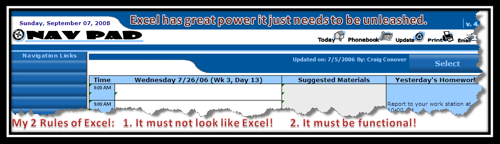
Here is an example that he gives:
Download now..............

Here is the Addin to make it happen in your spreadsheet. You will also need to put the code from the example into your spreadsheet and the form.
Download now

Improving Performance in Excel 2007

http://msdn2.microsoft.com/en-us/library/aa730921.aspx

Summary: Learn about the increased worksheet capacity in Microsoft Office Excel 2007 and techniques that you can use as you design and create worksheets to improve calculation performance. (40 printed pages)

Charles Williams, Decision Models Limited

October 2006

Applies to: Microsoft Office Excel 2007, Microsoft Office Excel 2003, Microsoft Excel 2002, Microsoft Excel 2000

Contents

• Overview

• The "Big Grid" and Increased Limits in Excel 2007

• Why Is Calculation Speed Important?

• Understanding Calculation Methods in Excel

• Calculating Workbooks, Worksheets, and Ranges

• Controlling Calculation Options

• Making Workbooks Calculate Faster

• Finding and Prioritizing Calculation Bottlenecks

• Excel 2007 Performance Improvements

• Tips for Optimizing Bottlenecks

• Workbook Opening, Closing, Saving, and Size

• Conclusion

• Additional Resources

Filename in cell

http://www.ozgrid.com/forum/showthread.php?t=53472

=REPLACE(LEFT(CELL("filename",A2),FIND("]",CELL("filename",A2))-5),1,FIND("[",CELL("filename",A2)),"")

or possibly better

=MID(CELL("filename"),SEARCH("[",CELL("filename"))+1,SEARCH("]",CELL("filename"))-5-SEARCH("[",CELL("filename")))